聚集层次算法
Python机器算法聚集层次算法详细操作教程
聚集层次算法简介
分层聚类是另一种无监督的学习算法,用于将具有相似特征的未标记数据点分组在一起。分层聚类算法分为以下两类。
聚集层次算法-在聚集层次算法中,每个数据点都被视为单个群集,然后依次合并或聚集(自下而上)群集对。群集的层次结构表示为树状图或树状结构。
分割分层算法-另一方面,在分割分层算法中,所有数据点都被视为一个大聚类,并且聚类的过程涉及将(大自上而下的方法)划分为一个大聚类聚集成各种小集群。
执行聚集层次聚类的步骤
我们将解释最常用和最重要的层次聚类,即聚类。执行相同的步骤如下-
第1步-将每个数据点视为单个群集。因此,开始时我们将拥有K个群集。开始时,数据点的数量也将为K。
第2步-现在,在这一步中,我们需要通过连接两个壁橱数据点来形成一个大集群。这将总共产生K-1个簇。
第3步-现在,要形成更多集群,我们需要加入两个壁橱集群。这将导致总共有K-2个集群。
第4步-现在,要形成一个大集群,请重复上述三个步骤,直到K变为0,即不再有要连接的数据点。
第5步-最后,在制作了一个大簇之后,将根据问题使用树状图将其分为多个簇。
树状图在聚集层次聚类中的作用
正如我们在最后一步中讨论的那样,一旦大集群形成,树状图就开始发挥作用。根据我们的问题,将使用树状图将群集分为相关数据点的多个群集。通过以下示例可以理解-
示例1
要了解,让我们从导入所需的库开始,如下所示:-
# Filename : example.py
# Copyright : 2020 By Lidihuo
# Author by : www.lidihuo.com
# Date : 2020-08-26
%matplotlib inline
import matplotlib.pyplot as plt
import numpy as np
接下来,我们将绘制本例中获取的数据点-
# Filename : example.py
# Copyright : 2020 By Lidihuo
# Author by : www.lidihuo.com
# Date : 2020-08-26
X = np.array(
[[7,8],[12,20],[17,19],[26,15],[32,37],[87,75],[73,85], [62,80],[73,60],[87,96],])
labels = range(1, 11)
plt.figure(figsize = (10, 7))
plt.subplots_adjust(bottom = 0.1)
plt.scatter(X[:,0],X[:,1], label = 'True Position')
for label, x, y in zip(labels, X[:, 0], X[:, 1]):
plt.annotate(
label,xy = (x, y), xytext = (-3, 3),textcoords = 'offset points', ha = 'right', va = 'bottom')
plt.show()
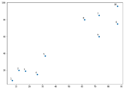
从上图很容易看出,我们在数据点外有两个集群,但在实际数据中,可以有成千上万个集群。接下来,我们将使用Scipy库来绘制数据点的树状图-
# Filename : example.py
# Copyright : 2020 By Lidihuo
# Author by : www.lidihuo.com
# Date : 2020-08-26
from scipy.cluster.hierarchy import dendrogram, linkage
from matplotlib import pyplot as plt
linked = linkage(X, 'single')
labelList = range(1, 11)
plt.figure(figsize = (10, 7))
dendrogram(linked, orientation = 'top',labels = labelList,
distance_sort ='descending',show_leaf_counts = True)
plt.show()
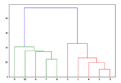
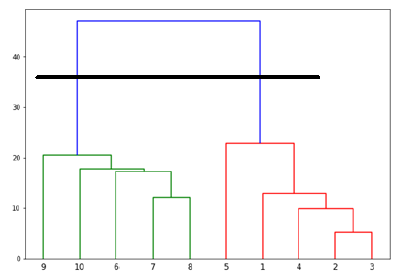
现在,一旦形成大簇,就选择了最长的垂直距离。然后通过一条垂直线绘制一条线,如下图所示。当水平线与蓝线在两个点处相交时,簇的数量将为两个。
接下来,我们需要导入用于聚类的类,并调用其fit_predict方法来预测聚类。我们正在导入
sklearn.cluster 库的
AgglomerativeClustering 类-
# Filename : example.py
# Copyright : 2020 By Lidihuo
# Author by : www.lidihuo.com
# Date : 2020-08-26
from sklearn.cluster import AgglomerativeClustering
cluster = AgglomerativeClustering(n_clusters = 2, affinity = 'euclidean', linkage = 'ward')
cluster.fit_predict(X)
接下来,在以下代码的帮助下绘制群集-
# Filename : example.py
# Copyright : 2020 By Lidihuo
# Author by : www.lidihuo.com
# Date : 2020-08-26
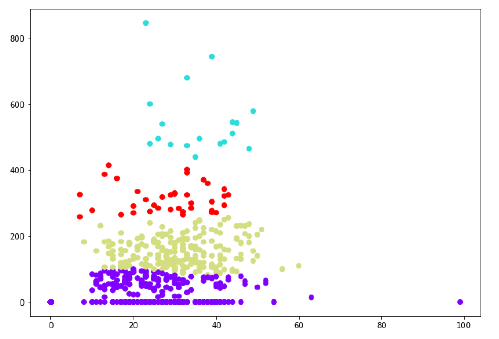
plt.scatter(X[:,0],X[:,1], c = cluster.labels_, cmap = 'rainbow')
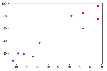
上图显示了来自我们数据点的两个群集。
示例2
正如我们从上面讨论的简单示例理解树状图的概念一样,让我们转到另一个示例,在该示例中,我们将使用分层聚类在Pima Indian Diabetes数据集中创建数据点的聚类。
# Filename : example.py
# Copyright : 2020 By Lidihuo
# Author by : www.lidihuo.com
# Date : 2020-08-26
import matplotlib.pyplot as plt
import pandas as pd
%matplotlib inline
import numpy as np
from pandas import read_csv
path = r"C:\pima-indians-diabetes.csv"
headernames = ['preg', 'plas', 'pres', 'skin', 'test', 'mass', 'pedi', 'age', 'class']
data = read_csv(path, names = headernames)
array = data.values
X = array[:,0:8]
Y = array[:,8]
data.shape
(768, 9)
data.head()
| |
Preg |
Plas |
Pres |
皮肤 |
测试 |
质量 |
Pedi |
年龄 |
类 |
| 0 |
6 |
148 |
72 |
35 |
0 |
33.6 |
0.627 |
50 |
1 |
| 1 |
1 |
85 |
66 |
29 |
0 |
26.6 |
0.351 |
31 |
0 |
| 2 |
8 |
183 |
64 |
0 |
0 |
23.3 |
0.672 |
32 |
1 |
| 3 |
1 |
89 |
66 |
23 |
94 |
28.1 |
0.167 |
21 |
0 |
| 4 |
0 |
137 |
40 |
35 |
168 |
43.1 |
2.288 |
33 |
1 |
# Filename : example.py
# Copyright : 2020 By Lidihuo
# Author by : www.lidihuo.com
# Date : 2020-08-26
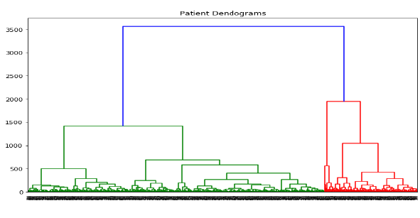
patient_data = data.iloc[:, 3:5].values
import scipy.cluster.hierarchy as shc
plt.figure(figsize = (10, 7))
plt.title("Patient Dendograms")
dend = shc.dendrogram(shc.linkage(data, method = 'ward'))
# Filename : example.py
# Copyright : 2020 By Lidihuo
# Author by : www.lidihuo.com
# Date : 2020-08-26
from sklearn.cluster import AgglomerativeClustering
cluster = AgglomerativeClustering(n_clusters = 4, affinity = 'euclidean', linkage = 'ward')
cluster.fit_predict(patient_data)
plt.figure(figsize = (10, 7))
plt.scatter(patient_data[:,0], patient_data[:,1], c = cluster.labels_, cmap = 'rainbow')