PyTorch线性回归
PyTorch线性回归详细操作教程
在本章中,我们将重点介绍使用
TensorFlow进行线性回归实现的基本示例。逻辑回归或线性回归是用于对离散类别进行分类的监督机器学习方法。在本章中的目标是构建一个模型,用户可以通过该模型预测预测变量与一个或多个自变量之间的关系。
如果y是因变量x而变化,则x认为是自变量。两个变量之间的这种关系可认为是线性的。两个变量的线性回归关系看起来就像下面提到的方程式一样 -
# Filename : example.py
# Copyright : 2020 By Lidihuo
# Author by : www.lidihuo.com
# Date : 2020-08-23
Y = Ax+b
接下来,我们将设计一个线性回归算法,有助于理解下面给出的两个重要概念 -
成本函数
梯度下降算法
下面提到线性回归的示意图,解释结果 -
# Filename : example.py
# Copyright : 2020 By Lidihuo
# Author by : www.lidihuo.com
# Date : 2020-08-23
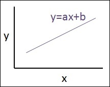
Y=ax+b
a的值是斜率。
b的值是y -截距。
r是相关系数。
r^2是相关系数。
线性回归方程的图形视图如下所述 -
以下步骤用于使用PyTorch实现线性回归 -
第1步
使用以下代码导入在PyTorch中创建线性回归所需的包 -
# Filename : example.py
# Copyright : 2020 By Lidihuo
# Author by : www.lidihuo.com
# Date : 2020-08-23
import numpy as np
import matplotlib.pyplot as plt
from matplotlib.animation import FuncAnimation
import seaborn as sns
import pandas as pd
%matplotlib inline
sns.set_style(style = 'whitegrid')
plt.rcParams["patch.force_edgecolor"] = True
第2步
使用可用数据集创建单个训练集,如下所示 -
# Filename : example.py
# Copyright : 2020 By Lidihuo
# Author by : www.lidihuo.com
# Date : 2020-08-23
m = 2 # slope
c = 3 # interceptm = 2 # slope
c = 3 # intercept
x = np.random.rand(256)
noise = np.random.randn(256) / 4
y = x * m + c + noise
df = pd.DataFrame()
df['x'] = x
df['y'] = y
sns.lmplot(x ='x', y ='y', data = df)
得到的结果如下所示:
第3步
使用PyTorch库实现线性回归,如下所述 -
# Filename : example.py
# Copyright : 2020 By Lidihuo
# Author by : www.lidihuo.com
# Date : 2020-08-23
import torch
import torch.nn as nn
from torch.autograd import Variable
x_train = x.reshape(-1, 1).astype('float32')
y_train = y.reshape(-1, 1).astype('float32')
class LinearRegressionModel(nn.Module):
def __init__(self, input_dim, output_dim):
super(LinearRegressionModel, self).__init__()
self.linear = nn.Linear(input_dim, output_dim)
def forward(self, x):
out = self.linear(x)
return out
input_dim = x_train.shape[1]
output_dim = y_train.shape[1]
input_dim, output_dim(1, 1)
model = LinearRegressionModel(input_dim, output_dim)
criterion = nn.MSELoss()
[w, b] = model.parameters()
def get_param_values():
return w.data[0][0], b.data[0]
def plot_current_fit(title = ""):
plt.figure(figsize = (12,4))
plt.title(title)
plt.scatter(x, y, s = 8)
w1 = w.data[0][0]
b1 = b.data[0]
x1 = np.array([0., 1.])
y1 = x1 * w1 + b1
plt.plot(x1, y1, 'r', label = 'Current Fit ({:.3f}, {:.3f})'.format(w1, b1))
plt.xlabel('x (input)')
plt.ylabel('y (target)')
plt.legend()
plt.show()
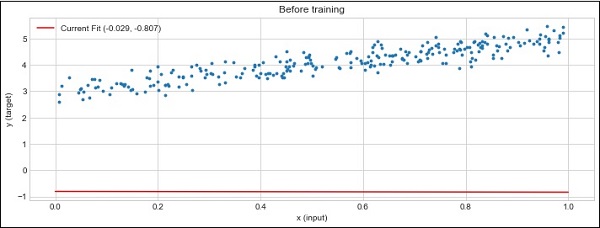
plot_current_fit('Before training')
执行上面示例代码,得到以下结果 -